Hi,
I want to create a table for interpolating saturation steam pressure in a PL controller. The PLC allows 120 setpoints that I can define individually. The PLC will do linear interpolation between the two nearest setpoints. I want to get the highest possible accuracy.

So how do I define the setpoints for temperature in order to get the best accuracy for saturation steam pressure?

I am aware that there might be more than one solution i.e. one for lowest absolute error and one for lowest relative error. However I do not have sufficient mathematical and Smath-specific knowledge to do it myself. I read about inverse distance weighting but what I need is somehow the opposite since I can choose the setpoints.

Attached is a sheet with the formula
Sattigungsdampfdruck-Stutzpunktberechnung.sm (13 KiB) downloaded 34 time(s).

IAPWS-97 is scalar. From a for loop, create/range your table.
wrt your PLC [Programmable Logic Controller]
ramp a linear SP over 120 elements. Next demo.
Please, confirm it works. Jean

Sattigungsdampfdruck-Stutzpunktberechnung.sm (38 KiB) downloaded 26 time(s).

Dear Jean
Thank you for the advice. I must admit I have difficulties understanding what you are saying. In your sheet I see an alternative formula for calculating saturation steam pressure. That was not what I was looking for.

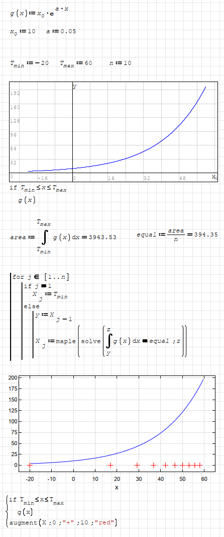
I am looking for a method that with a given formla E(t) for saturation steam pressure over temperature will return a list of interpolation points for temperature. I do not want do do this by trial and error since there are 120 parameters to vary. Once I have the list with temperatures I will run them through the formula e(t) thus creating a table with two rows one for t one for E and 120 columns.

This method assumes that the error in linear interpolation is related to the curvature. The problem is reduced from 120 parameters to just a few.
You still have to adjust them by hand, according to what your understanding of optimal distribution is. I tried to minimize the maximum absolute error.

Note that for 120 points, you probably need to increase the sampling points of the plot to not undersample the error.


Optimal sampling points_Kr.sm (28 KiB) downloaded 35 time(s).

Wrote

I am looking for a method that with a given formula E(t) for saturation steam pressure over temperature will return a list of interpolation points for temperature. I do not want do do this by trial and error since there are 120 parameters to vary. Once I have the list with temperatures I will run them through the formula e(t) thus creating a table with two rows one for t one for E and 120 columns.

You mean bar(°C) ... not anything E(t)
There is noting to solve wrt IAPWS-97
Construct the 120 pairs from a for loop.
Range 't' as you wish ... export to PLC.
Jean

At this point, as far as it might mean,
at each PLC scan, it will take the next 't,bar(t)'

Worksheet64 bar(degC).sm (27 KiB) downloaded 25 time(s).

The other perfect option is to establish the XFR of bar(°C)
XFR [Transfer Function]
Range at will over 120 points, plug in PLC.
XFR is the graphical representation of a system open loop
moving from steady state 0 to another state W/O oscillations
This is why the discrete XFR is the perfect option.
Jean

Thank you so much for your replies!

Especially the answer of Martin Kraska looks promising.

As far as I understand it is a major problem that the curve I used in the first row consists of two formulas. So it would be complicated to determine how many sampling points should be assigned to the low and high temperature range. Hence the idea of Jean Giraud is good to use a formula that is valid for the entire range in question. I integrated this IAPWS-97 formula in Martin Kraskas example.

I am not convinced that this question is too much about "taste". With a given assumption there should be a limited number of solutions. This is an optimisation problem. And I assume least squares would be the method to go. So I can either create a solution that minimizes absolute error (guess the unit would be Pa*K) and one that mininizes percentual (relative) error.

In Martins example I marked those parameters that are input as green. There remain four parameters that need calculation. One of them is determined by T.max but I do not see the formula for calculating h.0 out of T.max so any help appreciated.

The example below does not work because Smath cannot calculate the second derivative. I don't know why, this should be possible.

@Jean: H have not understood part of what you are trying to say. What are wrt and XFR? Then I think you have not understood what I am actually trying. I am looking for X in Martins example.

Again, thank you so much for the ideas provided!

Optimal sampling points_v2.sm (26 KiB) downloaded 34 time(s).

Wrote

The example below does not work because Smath cannot calculate the second derivative. I don't know why, this should be possible.

@Jean: H have not understood part of what you are trying to say. What are wrt and XFR? Then I think you have not understood what I am actually trying. I am looking for X in Martins example

Confirmed: IAPWS-97 does not support derivative.
If you discretize/spline, you can have first, 2nd, third, fourth derivatives
from infinitesimal analysis.
Forget XFR. IAPWS-97 not compatible Laplace.
On the other hand, you can populate from the code logpts
Jean

Wrote

@Jean: H have not understood part of what you are trying to say.

Don't bother, he doesn't have any intention to help you.
He is the master troll of this forum, the great nuisance.
Jean's only interest is promoting his worksheets.
Whether they are related with the question or not.
I really don't know the motivation behind it.
Is he getting paid per download of his samples?
I can't really tell, because he never posts anything useful.

Wrote

Confirmed: IAPWS-97 does not support derivative

So I guess we have to go back to Magnus formula which supports second order derivative.

The new sheet does not give an error anymore but still does not make sense nor does it show the error or solve an optimisation problem:

Optimal sampling points_v3.sm (25 KiB) downloaded 35 time(s).

Wrote

So I guess we have to go back to Magnus formula which supports second order derivative.

The new sheet does not give an error anymore but still does not make sense nor does it show the error or solve an optimisation problem:

You mean back to square one to your original demand; 2 rows of 120 cols
that you can plug in the PLC, all in ultimate accuracy.

Worksheet64 bar(degC).sm (27 KiB) downloaded 26 time(s).

@Jean: The sampling points in your example are evenly distributed. I already had such a table before I posted here. This is not what I need. The result of such a table is not of "ultimate accuracy" because the curve to be interpolated is much more curved on the high side. Second derivative (curvature) is about 64 times stronger at 60 °C than on -25 °C. Thus I need more points in the high temperature range.

Wrote

@Jean: The sampling points in your example are evenly distributed. I already had such a table before I posted here. This is not what I need. The result of such a table is not of "ultimate accuracy" because the curve to be interpolated is much more curved on the high side. Second derivative (curvature) is about 64 times stronger at 60 °C than on -25 °C. Thus I need more points in the high temperature range.

1. AFAIK,there is no known technical accuracy.
2. Split the ranges of your choice mesh at will, stack.

Inst_IAPWS region 1 DECADES.sm (53 KiB) downloaded 30 time(s).

Wrote

Thus I need more points in the high temperature range.

Could finding X positions which divide area under the curve into equal segments be the answer?
I am not a mathematician, just a simple engineer. Thus this reply can be totally wrong.
If so sorry for that priorly. I would really be ashamed if I made myself a fool.

PS: I couldn't make any solvers work while integral boundary is unknown.
For that, I used maple. And this made calculation very very slow.
If there is a faster and embedded way (no maxima), I would like to know.
Because I don't know.

Regards

area_divide.sm (9 KiB) downloaded 25 time(s).

Wrote

Could finding X positions which divide area under the curve into equal segments be the answer?

This would work only if the value of the function is proportional to it's curvature, e.g. exp(), sin().

In order to check the approach, make a plot of the error just like further above in my previous post.
Essentially, this is a minimax problem, where you want to minimize the maximum error. It should be sufficient to sample the error at the sampling points and in the center of the intervals.

Perhaps an evolutionary algorithm would be worth a try. The variables are the step sizes h_i. After each recombination/mutation step, you have to calibrate the h_i to enforce the boundary condition of the total x range.

Here is a version with evaluation of the error. This helps with setting the centering parameter.

There are two versions giving the same result.


Optimal sampling points_Kr.sm (44 KiB) downloaded 31 time(s).

Great, thank you so much Martin!

Your approach up to now had the disadvantage it only worked for positive Celsius temperatures. I made a version that fixes this. First I made symbolical calculation possible and simplified the function:


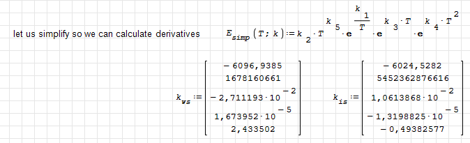
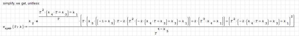
The challenge (for me) was to calculate the curvature symbolically. This was possible with some simplifications and the Maxima diff function instead of the built-in one.


Then I calculated the root mean square (RMS) error which can be minimised in a next step:


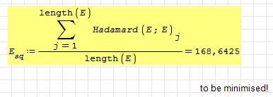
I think it is better to minimise the RMS error instead of the max error. For an engineering application anything bigger than T.max will be considered "big". So I don't care about the max. error too much as long as it is at one of the ends of the interpolation range.

For my final solution I can only enter the X values in °C with one decimal place. This will have a minor impact on the result. That's why I added a rounding function.

What I did not understand in the sheet above is why you calculate E(X) twice. Is that just an alternate approach?

How do I do the actual optimisation?

Optimal sampling points_Kr-bj.sm (67 KiB) downloaded 32 time(s).

Nice to see successful applications of Maxima

The two implementations of E(X) give the same result. I added the if-based one because it might be easier to understand. Not everyone is familiar with convolutions.

I wonder why you put a lot of effort in minimizing the error and then being satisfied with some RMS instead of a rigid bracketing. I am not sure at all that I understand your concept of error.

As to the optimization: Do you have to solve multiple such problems or just this one? In the latter case just be pragmatic and play around with the parameters until you are satisfied. There is next to nothing an optimizer could gain in the given example.

As I said, for a general solution I'd skip the curvature based approach and use brute force evolutionary algorithm.

Wrote

Your approach up to now had the disadvantage it only worked for positive Celsius temperatures. I made a version that fixes this. First I made symbolical calculation possible and simplified the function:

Below the triple point of Water [0.01°C], the function is ice sublimation.
Exists in Smath from source, down to -90 °C

Wrote

I wonder why you put a lot of effort in minimizing the error and then being satisfied with some RMS instead of a rigid bracketing. I am not sure at all that I understand your concept of error.

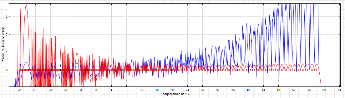
In an engineering application it's generally more about relative error instead of absolute error. I modified your example in order to show relative error and surprisingly the needed exponent p becomes negative! Means I need more points in the low temperature range than in the high temperature range. Blue is absolute error, red is relative error:

Wrote

As to the optimization: Do you have to solve multiple such problems or just this one? In the latter case just be pragmatic and play around with the parameters until you are satisfied. There is next to nothing an optimizer could gain in the given example.

I don't have many problems like this. I would like to do another one for the inverse function and one for the derivative. But I agree that for this purpose the room for optimisation is small. The red curve is amplified by 1000 so I have a peak error of 3.7 ‰ at the end and average errors less than 0.5 ‰ in the middle range. In order to further improve I would have to reduce the discretization error but that would require different hardware.

This was an interesting exercise I enjoyed much, thanks for contributing!

Optimal sampling points_Kr-bj2.sm (60 KiB) downloaded 34 time(s).