Both ranges from my expertise in data fitting.
The long range [Thiele continued fraction] has
anothr form of J_Fraction but not much to gain.
Excel digests continued fractions, code carefully.

Jean

Inst_Viscosity Water.sm (24 KiB) downloaded 85 time(s).

Looks like this is at the pressure just above saturation.

Wrote

Looks like this is at the pressure just above saturation.

One remarkable continued fraction is the air ρ/km altitude.
I always wondered why so few physical phenomenons are quadratic
vs so many are hyperbolic. Maybe, I didn't live long enough !


Cheers, Jean.

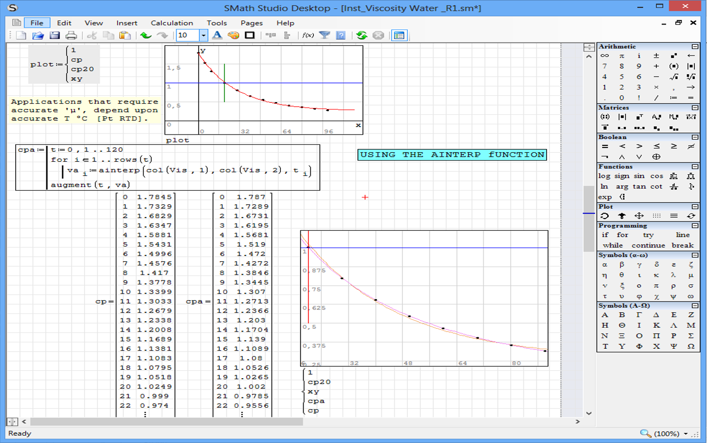
I think for more precision in the calculation of viscosity of water , you should use the interpolation function " ainterp " , applying it directly to the table.

Inst_Viscosity Water _R1.sm (39 KiB) downloaded 40 time(s).

Best Regards

Wrote

I think for more precision in the calculation of viscosity of water , you should use the interpolation function " ainterp " , applying it directly to the table.

That's incorrect.
1. Tabular data is itself approximation. There's no need to match it exactly.
2. Jean's method is much faster. If high scientific precision is required, then CoolProp wrapper could be used, but it solves about 2x longer (being binary optimized library!) than Jean's method.
3. Jean's gives much better extrapolation.


==

And last, but not least: this is not only a tool, but also a great example and lesson of high-quality data fitting.

There are several answers "à la carte"
1. ainterp is particular to Smath and not same kind of cubic "cinterp" which is universal
[Smath = Mathcad = Matlab = Mathematica = OriginLab = Maple ... tracable to "Numerical Recipes"].
Also same as ACM. l_p_c splines have been posted in "Samples".
2. Cubic splines are for sparse points that have no physical meaning.
3. Viscosity is a smooth physical phenomenon, not of polynomial format. Therefore not representable
by cubic pieces or from any higher nth order pieces. Cubic splines are not monotonous, they wiggle
between points.
4. The matter is not if one data set is better than another one, no: the matter is a smooth analytical
representation, tracable to the source. Interpolation instead of a model function is erroneous. Would
you interpolate for sin(x), sure not.
5. The long range 0 °C ... critical point, the data set is sourced from IAPWS. The continued fraction,
you will find nowhere else than in Smath and in my old Mathcad 11 web collection "mathengjmg". I have
another representation that requires a bit of Smath program [works well].
6. Both ranges you can plug in your pocket calculator and go hunting. Or pass to team work that don't
have Smath. Both ranges work fine in Excel, Matlab, OriginLab, Mathematica ... because they are mathh
tools capable of executing the code.
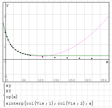
7. The short range has another Decay representation. It elongates the formula for little gain. I suppose
that if you are in that range of 100 °C, you will need above as well: then use the total range 0.. critical.
8. Unless you plot and appreciate the trend, don't extrapolate cubic splines, especially the Smath cinterp.
Depending upon the trend, the lspline maybe better at one end or another... or maybe the pspline.

Cheers, Jean