Bonjour Jean Giraud

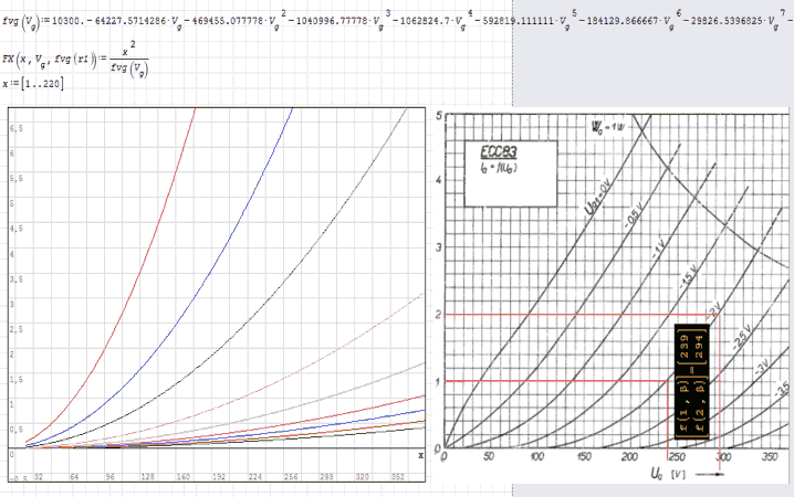
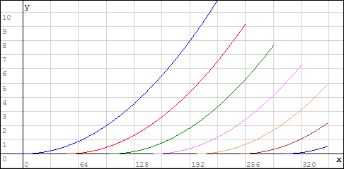
Koren's equations are "phenomenological", that is, following a certain succession of phenomena. Almost always, however, mathematical models have accompanied some simplified physical models for various reasons. If we look especially at the characteristic curves corresponding to the pentodes and the tetrods, we will observe that quite often the characteristic curves are no longer strictly monotonous, as the so-called phenomenological equation, but also contain negative slope portions with the reversal of monotony. Thus, for the EL34 power pentode, it can be seen from the diagram on page 11 of this document that for command line voltages more negative than 20 V, the curves have some very strange evolutions. That's the way things stand, the phenomenological equations must remain open to various innovative changes if their charts can be made to reproduce as accurately as possible the curves automatically drawn in the labs.

Hola Carlos

To have access to the file you have linked to, you must become a member of that forum. I have almost a horror of forums. With the exception of SMath Studio Forum, which I have enrolled to benefit from the advice of the users of this CAD program, I am only a member of two forums. One of them (where I have been a moderator for nearly 6 years) posts less and less because of the exacerbat radicalism of many of its members. The other, with fewer members, does not yet have this phenomenon and participates in discussions, but mostly publicly various technical articles. To one of these articles, you have a link in a previous post.

Otherwise, the best of both.

Nicolas

Bonjour Nicolas,

No need to login to the forum you are referencing. Polynomials have nothing
to do in physics, they are just casual convenient gadgets. But this is not
true in mathematics, all maths functions are approximated by normalised
rational fraction i.e: rational fraction of polynomials.

Let's stay on the triode from lab experiment of high quality measurements.
What comes in comes out TRNSFORMED. The physics between the in-out is
strictly and nothing else than the XFR [Transfer Function]. That it is
pure or imperfect depends upon the dynamics of the system. Koren's formula
is empirical for convenient representation. In the stable range of the dynamics
it has as single form of XFR for 6 curves. Each curve is simply the XFR shifted.

The notion of XFR governs modeling control systems, easy since advanced CAS.
Before the modern numerical, modeling was done from "Analog Computers"
Typical system was Systron Doner, now museum.

1. Setup your lab experiments [Hi Pro.]
2. Collect enough raw measured values.
3. Collect the mA vs Volts in Smath data vectors
4. Attach in Smath Forum ... Jean will be delighted working that stuff.

Experiment the Explorer [2 ... 7]

A bientôt Nicolas with your data sets ... Jean.

0Appendix_00000 TESLA Models Copy.sm (80 КиБ) скачан 40 раз(а).

Bună ziua Nicolas

Registration is not required on the page. The file can be downloaded directly from:




salutări


Hello Jean

I believe that the function should be something similar to what I show here.
This attempt is only an idea, where the equation only depends on the value Ua and Ug.





Tesla_Origen_CBG_Jean.sm (122 КиБ) скачан 40 раз(а).


regards

Carlos

Thanks both for your greetings

I see that now the link posted by Carlos to message # 39 has been opened. But there is a list of links. Which one leads to the excel document? ...

... It's okay, I found it.

Wrote

...
1. Setup your lab experiments [Hi Pro.]
2. Collect enough raw measured values.
3. Collect the mA vs Volts in Smath data vectors
4. Attach in Smath Forum ... Jean will be delighted working that stuff.

Hello Jean Giraud

I wish I had enough time for all this. Like in my youth, I was able to do more than now. Maybe after I retire.

Nicolas.

Wrote

Maybe after I retire.

Oh ! Nicolas, don't wait you retire. By the time, I will be sucking the roots!
Carlos: does it make sense to recast with more flexibility [typical] ?

Jean



Project Tesla_Origen_CBG_Jean.sm (137 КиБ) скачан 50 раз(а).

Greetings

I do not know what "r1" is in Carlos's relationship. And then what I see does not correspond visually to the diagrams in the datasheet.
... And what about the first curve?



Nicolas

Wrote

I do not know what "r1" is in Carlos's relationship. And then what I see does not correspond visually to the diagrams in the datasheet.
... And what about the first curve?

1. The parameter 'r1' is not accounted ... removed
2. This is experimental from observed ... your data set is phenomenological.
So, they don't relate. You had the XFR phenomenological from before.
3. "first curve" is not experimental ... a fake one added.

Jean

Project Tesla_Origen_CBG_Jean [Refactored].sm (11 КиБ) скачан 44 раз(а).

Hello

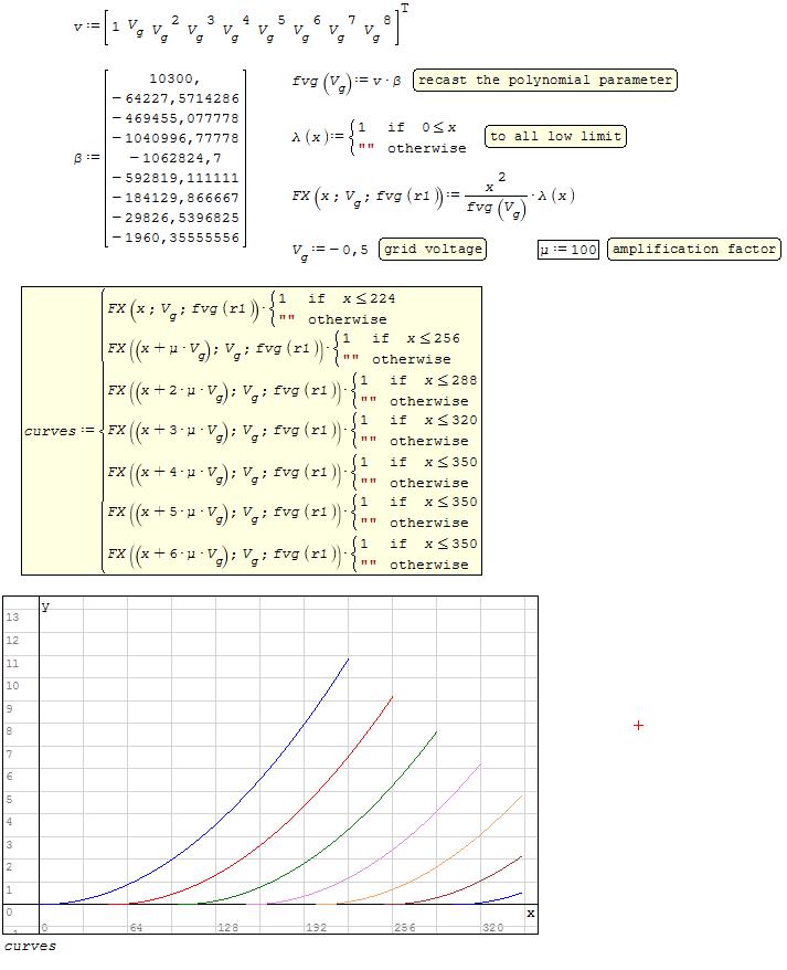
Very good. Let's say that in the file attached to you, we have the desired shape of the curves. Basically, I only got a beam of curves similar to those in the datasheet. How do I now define the unique function that will generate for each pair of Va and Vg variables the Static Operating Point (SOP)? I do not really need a picture of the characteristic curves, but a relationship that generates for each couple of input data a single SOP in the voltage-current plane. In other words, we look at the variable Vg as one that takes values in a continuous domain, and not a sequence of predetermined values. As I have already mentioned, the mathematical model is going to be useful in a simulation program.

Nicolas

Hello everybody

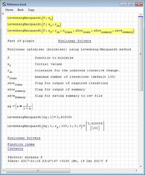
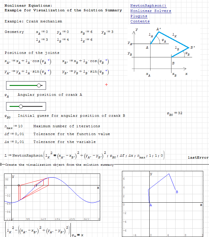
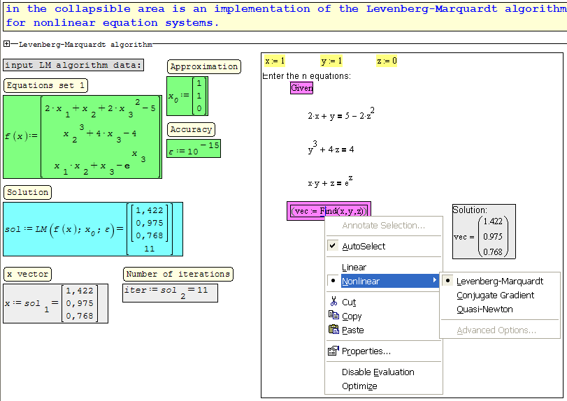
The Levenberg-Marquardt method can be (I hope) closely related to solving the non-linear equation system that interests me. In SMath, however, there are seven different variants of the Levenberg-Marquardt method. I think I understand what it is about LevenbergMarquardt (2) and LevenbergMarquardt (3). I ask someone to explain what are the input sizes for the variants: LevenbergMarquardt (7); LevenbergMarquardtCD (2); LevenbergMarquardtCD (3); LevenbergMarquardtCD (4) and LevenbergMarquardtCD (8). Small examples of application would be very useful. All the best.

Nicolas

Wrote

The Levenberg-Marquardt method can be (I hope) closely related to solving the non-linear equation system that interests me

Davide will help you on that, I think he is the creator.
NOW: don't confuse with the Mathcad Minerr LM, which is
a specific tool to fit model function(s) to data sets.
Mathcad Minerr LM is a proprietary Mathsoft code, never
published or hinted. I wish it could be implemented
in Smath. Alternately, we have Conjugate Gradient,
lot more difficult to initialize.

Sorry Nicolas, can't help ... Jean

Wrote

Hello everybody

The Levenberg-Marquardt method can be (I hope) closely related to solving the non-linear equation system that interests me. In SMath, however, there are seven different variants of the Levenberg-Marquardt method. I think I understand what it is about LevenbergMarquardt (2) and LevenbergMarquardt (3). I ask someone to explain what are the input sizes for the variants: LevenbergMarquardt (7); LevenbergMarquardtCD (2); LevenbergMarquardtCD (3); LevenbergMarquardtCD (4) and LevenbergMarquardtCD (8). Small examples of application would be very useful. All the best.

Nicolas

Try the interactive handbook.

Goto Functions Index, open the L area and Ctrl-Click to LevenbergMarquardt(). In the Nonlinear Solvers page you find a link on how to visualize the solution history.

Hello mkraska.

Thank you very much

Nicolas

Hello everybody

I have tried to write an algorithm in SMath to solve systems with several equations. In the attachment I have illustrated how with this algorithm I managed to solve the equation system given as an example in QuickSheets in MathCAD. I also provided the SMath file in the second attachment. Using the same algorithm I then tried to solve the problem defined in message # 1 of this topic - see the SMath file in attachment 3. After 7 iterations, the loop while from the algorithm comprised in the collapsible area became an infinite loop because size Δp has an error and the program perceives it as indefinite, although calculated separately the right member of the equation that on Δp has a finite value. I have set the spreadsheet for this file without using automatic calculation, because the higher the computing time, the computer's system memory resources are becoming less and less programmatic and the program tends to block the system. In program, the mm size set to mm = 1 corresponds to a current expressed in mA, while set to mm = 0.001 resulting streams will be scaled to Amps. To run the file, use the "Recalculate page" command in the "Calculation" toolbar, after which it will stop running after the first 20 ... 30 minutes. As the personal observations I could make, the variable vector does not change locally after 7 iterations, and the damping factor μ has a value very close to zero. Not being very experienced in such algorithms, I can not figure out where the wrong is. Perhaps the others will try to solve with me such a problem, which they will take as a challenge. Otherwise, good luck to everyone.

Nicolas

About Levenberg-Marquardt algorithm.sm (44 КиБ) скачан 41 раз(а).
About Levenberg-Marquardt algorithm_.sm (58 КиБ) скачан 44 раз(а).

Hello,

Unfortunately, numerically solving the system of more than few nonlinear equations is quite a problematic thing to do in SMath. After all these years I think this is one of the thing that will never be resolved in SMath in an efficient way.

Regards,
Radovan

Wrote

Hello,

Unfortunately, numerically solving the system of more than few nonlinear equations is quite a problematic thing to do in SMath. After all these years I think this is one of the thing that will never be resolved in SMath in an efficient way.

Regards,
Radovan

Modifications to the Levenberg-Marquardt Method
To make the Levenberg-Marquardt method more effective on actual problems, Mathcad includes the following modifications to the basic method:

The first time the solver stops at a point that is not a solution, Mathcad adds a small random amount to all the variables and tries again. This helps avoid getting stuck in local minima and other points from which there is no preferred direction. Mathcad does this only once per solve, the first time the solver stops on a point that is not a solution.

If you include inequality constraints in a solve block, Mathcad solves the subsystem consisting of only
the inequalities first before adding in the in the equality constraints and attempting a full solution.
This is equivalent to moving the guesses into an area where the inequalities are all satisfied before
starting the solver.

Solve GivenFind MCD Example.sm (10 КиБ) скачан 48 раз(а).

Wrote

I can not figure out where the wrong is.

Seemingly, you are trying to fit some data point to an infinitely modifiable model.
That is the wrong approach. Mathcad would surely complain !
Your LM MCD reports "Not Scalar" [6179]
Versions past 6179 are just pest, particularly 6671
Smath has fitted gorgeous more than 50 models/data sets.
Just give your data set, I will try.

Wrote

I can not figure out where the wrong is.

You can fit individually.
Not enough points to confirm a possible model.

Hello everyone.

@Radovan: I tried to reduce the system to a maximum of 3 equations with 3 unknowns, by replacing them with some acceptable constants. One of the unknown is even the one at the exponent. I thought this would reduce the difficulty of the problem. The algorithm behaves the same as for the 6 unknown 6 equations in the file I attached above. I deduce that the problem is somewhere else.

Wrote

... Seemingly, you are trying to fit some data point to an infinitely modifiable model. That is the wrong approach. Mathcad would surely complain ! ...

I did not even think about it, Jean Giraud. The algorithm used in my files above is the fruit of my own efforts. I built it by consulting a large bibliography in the field, as I am not a mathematics researcher. In principle, the guidelines of this algorithm are those in the article published here. From MathCAD, I only took the example. It was the most handy of all the possible examples, because it was practically ready.

Wrote

@Radovan: I tried to reduce the system to a maximum of 3 equations with 3 unknowns, by replacing them with some acceptable constants. One of the unknown is even the one at the exponent. I thought this would reduce the difficulty of the problem. The algorithm behaves the same as for the 6 unknown 6 equations in the file I attached above. I deduce that the problem is somewhere else

I appreciate your efforts in making a LM function by yourself. It will help you to understand and use the programming aspects of Smath. However, if your primer goal is to solve the system of nonlinear equations the simplest way might be to use the functions SMath has to offer you. For example, see the available functions in NonlinearSolvers plugin by Davide Carpi. Actually, Martin already suggests to you in the previous post to try this, although there is a chance that you would not be able to use most of the functions there because this is still a work in progress for a long time.

Regards,
Radovan