There is also an old example. This system reflects a real physical process. As far as I remember, it is connected with electricity.
It would be nice to show the complete solution, or an approach to obtaining the complete solution.

1 - 2cos(x1) + 2cos(x2) - 2cos(x3) - x4 = 0;
1- 2cos(5x1) + 2cos(5x2) - 2cos(5x3) = 0;
1 - 2cos(7x1) + 2cos(7x2) - 2cos(7x3) = 0;

Wrote

Wrote

40 solutions can be found

Hello Alvaro! Yes, thanks for the work done. This was, one might say, a test example for the Method. This system of equations has 116 solutions. The first two equations describe a closed curve; moving along it, we track the change in the sign of the last equation. There are 116 solutions in total.

The 116 solutions.



DraghilevSolveBlock - alexey 116 example.sm (275 КиБ) скачан 37 раз(а).

Wrote

There is also an old example. This system reflects a real physical process. As far as I remember, it is connected with electricity.
It would be nice to show the complete solution, or an approach to obtaining the complete solution.

1 - 2cos(x1) + 2cos(x2) - 2cos(x3) - x4 = 0;
1- 2cos(5x1) + 2cos(5x2) - 2cos(5x3) = 0;
1 - 2cos(7x1) + 2cos(7x2) - 2cos(7x3) = 0;

Do you have some other information? Like what is x4 (a parameter for making a lot of 3x3 nonlinear equations system?) Or how many solutions are, or something else.

Best regards.
Alvaro.

Wrote

Do you have some other information? Like what is x4 (a parameter for making a lot of 3x3 nonlinear equations system?) Or how many solutions are, or something else.

Yes, for a specific task x4 can be considered as something like a parameter. But the beauty of the system is precisely in this form. In other words, the real system became the basis for this one.
Also, please excuse me, I do not own or use SMath Studio. I think I can perceive the algorithm (idea of the solution) in words. If it's not difficult for you, of course. And, if you want, I will share my approach to solving it.

Wrote

Wrote

Do you have some other information? Like what is x4 (a parameter for making a lot of 3x3 nonlinear equations system?) Or how many solutions are, or something else.

Yes, for a specific task x4 can be considered as something like a parameter. But the beauty of the system is precisely in this form. In other words, the real system became the basis for this one.
Also, please excuse me, I do not own or use SMath Studio. I think I can perceive the algorithm (idea of the solution) in words. If it's not difficult for you, of course. And, if you want, I will share my approach to solving it.

Hi Alexey. Thanks, but I think the complete solution to this problem is out of my reach. The phenomenon seems to be quasiperiodic and the solutions have no limit and extend throughout space. Another difficulty is visualizing the 3 intersecting surfaces.

On the other hand, from the point of view of numerical methods the mathematical problem is reduced to finding an adequate solver for the differential equation given by D(t,u) = D which also exceeds my abilities for looking an specialized ODE solver given the complexity of the expression.



DraghilevSolveBlock - alexey elec example.sm (303 КиБ) скачан 43 раз(а).

Best regards.
Alvaro.

Hello Alvaro.
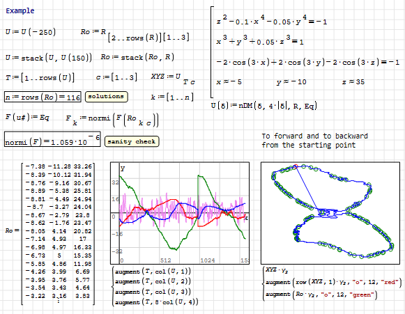
I think that in this case it is not very convenient to immediately apply Draghilev’s method. I tried two ways to get the solution. One way is to work directly with the system itself, that is, add some equation to the system to get the starting point, for example x1+x2+x3+x4=0. After this, we calculate the line in R^4. This line will be one of the subsets of the system solution. The coordinates of points x1, x2, x3 with a period of 2Pi will define an infinite set of subsets with coordinate x4. By changing the additional equation, we can get an idea of the set of such subsets. They are all solutions of the system.
Since the solution is numerical, it is probably impossible to say that we have found a complete solution. But practically it is possible.
As for visualization, we can display on a graph a combination of 3 coordinates out of 4: x1,x2,x3; x1,x2,x4: x1,x3,x4; x2,x3,x4. (This produces an infinite set of closed curves.)

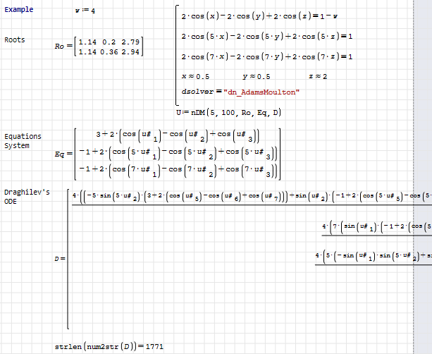
The second way is to reduce the original system to a system of polynomial equations by means of the following replacement

cos(x1) = x1, cos(x2) = x2, cos(x3) = x3.

1-2*x1+2*x2-2*x3-x4 = 0
-32*x1^5+32*x2^5-32*x3^5+40*x1^3-40*x2^3+40*x3^3-10*x1+10*x2-10*x3+1=0
-128*x1^7+128*x2^7-128*x3^7+224*x1^5-224*x2^5+224*x3^5-112*x1^3+112*x2^3-112*x3^3+14*x1-14*x2+14*x3+1=0

In this case, we get more opportunities to identify all the original subsets of solutions, because for any one auxiliary equation, according to the theory, all solutions are found (Gröbner bases). Then we make a reverse replacement, take into account the period, look at the graphs and, on a practical basis, assert that we have obtained a solution to the original system.
It's definitely a lot easier for me because Maple does all the work for me. Both Gröbner bases and powerful procedures for solving ODEs are implemented there. It takes literally seconds to obtain a solution in the form of a set of curves.

Wrote

Another difficulty is visualizing the 3 intersecting surfaces.

Of course, because SMath does not have the corresponding functions.

Wrote

Hello Alvaro! Yes, thanks for the work done. This was, one might say, a test example for the Method. This system of equations has 116 solutions. The first two equations describe a closed curve; moving along it, we track the change in the sign of the last equation. There are 116 solutions in total.

The zeros are obtained by linear interpolation of all 116 solutions.
Файл не найден.Файл не найден.

Wrote

I think the complete solution to this problem is out of my reach

Alvaro, if you're interested, I can share Maple's texts with you. The texts, of course, are not at a programmer level, but for the Method and the specific task they are quite understandable. For example, this can be done through my VK profile. Or suggest your own way.

Wrote

There is also an old example. This system reflects a real physical process. As far as I remember, it is connected with electricity.
It would be nice to show the complete solution, or an approach to obtaining the complete solution.

1 - 2cos(x1) + 2cos(x2) - 2cos(x3) - x4 = 0;
1- 2cos(5x1) + 2cos(5x2) - 2cos(5x3) = 0;
1 - 2cos(7x1) + 2cos(7x2) - 2cos(7x3) = 0;

Initial coordinates (x1,x2,x3,x4) : 7.3307 1.4976 1.4979 9.8840e-04
Файл не найден.Файл не найден.

Some solutions to check out:

5.7082e+00 2.0944e+00 2.5666e+00 -2.3061e-04
5.7076e+00 2.0944e+00 2.5660e+00 -2.2976e-04
5.7070e+00 2.0944e+00 2.5654e+00 -2.2892e-04
5.7063e+00 2.0944e+00 2.5647e+00 -2.2809e-04
5.7057e+00 2.0944e+00 2.5641e+00 -2.2728e-04
5.7051e+00 2.0944e+00 2.5634e+00 -2.2647e-04
5.7044e+00 2.0944e+00 2.5628e+00 -2.2567e-04
5.7037e+00 2.0944e+00 2.5621e+00 -2.2488e-04
5.7031e+00 2.0944e+00 2.5614e+00 -2.2410e-04
5.7024e+00 2.0944e+00 2.5608e+00 -2.2334e-04
5.7017e+00 2.0944e+00 2.5601e+00 -2.2258e-04
5.7010e+00 2.0944e+00 2.5594e+00 -2.2183e-04
5.7003e+00 2.0944e+00 2.5587e+00 -2.2109e-04
5.6996e+00 2.0944e+00 2.5580e+00 -2.2036e-04
5.6989e+00 2.0944e+00 2.5573e+00 -2.1964e-04
5.6982e+00 2.0944e+00 2.5565e+00 -2.1893e-04
5.6974e+00 2.0944e+00 2.5558e+00 -2.1822e-04
5.6967e+00 2.0944e+00 2.5551e+00 -2.1753e-04
5.6959e+00 2.0944e+00 2.5543e+00 -2.1684e-04
5.6952e+00 2.0944e+00 2.5536e+00 -2.1617e-04
5.6944e+00 2.0944e+00 2.5528e+00 -2.1550e-04

Wrote

Wrote

I think the complete solution to this problem is out of my reach

Alvaro, if you're interested, I can share Maple's texts with you. The texts, of course, are not at a programmer level, but for the Method and the specific task they are quite understandable. For example, this can be done through my VK profile. Or suggest your own way.

Hi Alexey. I only use Maple v 11, which actually runs on Windows 98 and with classic worksheets. This is because it is very easy to install and to explain the software in class without losing almost any of the computing power. I think my email is public in this forum: it is razonar at outlook dot com. The method I use for Draghilev's method is based on the procedure that Viacheslav posted somewhere here on the forum. The main modification was to optimize it for two or three variables, and subsequently change the way of entering the time span and the initial conditions.

Best regards.
Alvaro.

Wrote

Some solutions

Да, правильно, это часть одного из подмножества решений. И по первым трём переменным период 2Pi.

Wrote

I think my email is public in this forum

Okay, Alvaro, now I see your address. Let's do what we can, then I will gradually send my programs according to the Method. And let's see if it works on your version. It would be even better if you became a member of MaplePrimes. There on the forum, if necessary, they will help with the correct execution of the procedure on Maple. They are extremely professional and usually have a lot of useful information.
The first letter was sent...

Wrote

Hello Alvaro.
I think that in this case it is not very convenient to immediately apply Draghilev’s method. I tried two ways to get the solution. One way is to work directly with the system itself, that is, add some equation to the system to get the starting point, for example x1+x2+x3+x4=0. After this, we calculate the line in R^4. This line will be one of the subsets of the system solution. The coordinates of points x1, x2, x3 with a period of 2Pi will define an infinite set of subsets with coordinate x4. By changing the additional equation, we can get an idea of the set of such subsets. They are all solutions of the system.
Since the solution is numerical, it is probably impossible to say that we have found a complete solution. But practically it is possible.
As for visualization, we can display on a graph a combination of 3 coordinates out of 4: x1,x2,x3; x1,x2,x4: x1,x3,x4; x2,x3,x4. (This produces an infinite set of closed curves.)

The second way is to reduce the original system to a system of polynomial equations by means of the following replacement

cos(x1) = x1, cos(x2) = x2, cos(x3) = x3.

1-2*x1+2*x2-2*x3-x4 = 0
-32*x1^5+32*x2^5-32*x3^5+40*x1^3-40*x2^3+40*x3^3-10*x1+10*x2-10*x3+1=0
-128*x1^7+128*x2^7-128*x3^7+224*x1^5-224*x2^5+224*x3^5-112*x1^3+112*x2^3-112*x3^3+14*x1-14*x2+14*x3+1=0

In this case, we get more opportunities to identify all the original subsets of solutions, because for any one auxiliary equation, according to the theory, all solutions are found (Gröbner bases). Then we make a reverse replacement, take into account the period, look at the graphs and, on a practical basis, assert that we have obtained a solution to the original system.
It's definitely a lot easier for me because Maple does all the work for me. Both Gröbner bases and powerful procedures for solving ODEs are implemented there. It takes literally seconds to obtain a solution in the form of a set of curves.

Wrote

Another difficulty is visualizing the 3 intersecting surfaces.

Of course, because SMath does not have the corresponding functions.

Do I need also make replacement for left part of differential equation?
Something like that
cos(x1) = y1
dy1/dt=dcos(x1)/dt
dy1/dt=-sin(x1)*dx1/dt
dy1/dt=-sqrt(1-y^2)*dx1/dt
dx1/dt=-1/sqrt(1-y^2)*dy1/dt

Wrote

Do I need also make replacement for left part of differential equation?

Unclear. If you want to replace cos(x1) with y1, then in your original equation instead of cos(x1) you will simply have y1. And you solve a completely different system of equations, and that’s it, and then, after receiving the solution, you do the inverse transformation through arccos(y1). Just don’t forget what the arccos range is.
I made the substitution because for polynomial equations all the solutions are found in theory, and therefore it is very easy to work with the auxiliary equation. And the Method was applied to the resulting system after replacement.

(Непонятно. Если ты хочешь заменить cos(x1) на y1, то у тебя в исходном уравнении вместо cos(x1) будет просто y1. И ты решаешь уже совсем другую систему уравнений и именно её, а потом, после получения решения, делаешь обратное преобразование через arccos(y1). Только надо не забыть, какова область значений arccos.
Я делал замену, потому что для полиномиальных уравнений находятся все решения по теории, и поэтому очень легко работать со вспомогательным уравнением. И Метод я применял к получившейся после замены системе.)

Wrote

Wrote

Do I need also make replacement for left part of differential equation?

(Непонятно. Если ты хочешь заменить cos(x1) на y1, то у тебя в исходном уравнении вместо cos(x1) будет просто y1. И ты решаешь уже совсем другую систему уравнений и именно её, а потом, после получения решения, делаешь обратное преобразование через arccos(y1). Только надо не забыть, какова область значений arccos.
Я делал замену, потому что для полиномиальных уравнений находятся все решения по теории, и поэтому очень легко работать со вспомогательным уравнением. И Метод я применял к получившейся после замены системе.)

Меня смущает, что в новой системе нет никаких ограничений на значение косинусов. Ведь если их модуль больше единицы, мы получим комплексные числа. Решение исходной системы находится в вещественной области.

Wrote

Ведь если их модуль больше единицы, мы получим комплексные числа. Решение исходной системы находится в вещественной области.

Вот, заодно и проверишь, где они находятся. Бери готовую подстановку, которую я привёл.

[RUS]В новой системе, где произведена замена cos(xi) на xi, часть решений совпадает с исходной системой на некотором участке при cos меньших единицы. При значениях больше единицы получаем отклонения от исходной системы и комплексные числа, которые тоже являются решениями в исходной системе. Кружочком обозначил точку, где начинается отклонение.[/RUS]
[ENG]In the new system, where cos(xi) has been replaced by xi, part of the solutions coincide with the original system at some part at cos less than unity. For values greater than one, we obtain deviations from the original system and complex numbers, which are also solutions in the original system. The circle indicates the point where the deviation begins.[/ENG]
Файл не найден.Файл не найден.Файл не найден.Файл не найден.
Some solutions to check out:
0 + 0.405718i 0 + 0.392443i 0.261484 -0.943054
0 + 0.405880i 0 + 0.392625i 0.261456 -0.943057
0 + 0.406042i 0 + 0.392806i 0.261427 -0.943061
0 + 0.406205i 0 + 0.392988i 0.261399 -0.943065
0 + 0.406367i 0 + 0.393169i 0.261370 -0.943069
0 + 0.406529i 0 + 0.393351i 0.261342 -0.943072
0 + 0.406691i 0 + 0.393532i 0.261313 -0.943076
0 + 0.406853i 0 + 0.393713i 0.261285 -0.943080
0 + 0.407015i 0 + 0.393895i 0.261256 -0.943083
0 + 0.407177i 0 + 0.394076i 0.261228 -0.943087
0 + 0.407339i 0 + 0.394257i 0.261200 -0.943091
0 + 0.407501i 0 + 0.394438i 0.261171 -0.943095
0 + 0.407662i 0 + 0.394618i 0.261143 -0.943098
0 + 0.407824i 0 + 0.394799i 0.261115 -0.943102
0 + 0.407986i 0 + 0.394980i 0.261087 -0.943106
0 + 0.408147i 0 + 0.395160i 0.261059 -0.943110
0 + 0.408309i 0 + 0.395340i 0.261030 -0.943113
0 + 0.408470i 0 + 0.395521i 0.261002 -0.943117
0 + 0.408631i 0 + 0.395701i 0.260974 -0.943121
0 + 0.408793i 0 + 0.395881i 0.260946 -0.943124
0 + 0.408954i 0 + 0.396061i 0.260918 -0.943128

[albumimg]1704[/albumimg]

0.468662334900000, -0.505048076100000, -0.983806563200000, 1.02019230400000
0.278151371288816, -0.646641165036486, -0.958295562906639, 1.06700605276267
0.187740508428832, -0.621552611483207, -0.957035692786738, 1.29548514534940
0.123989711411092, -0.571693315241923, -0.961666058174577, 1.53196606264312
0.0627943321172479, -0.517036824844165, -0.963882589079057, 1.76810286383529
0.00303231822847996, -0.458188604728475, -0.963024061229262, 2.00360627614461
-0.0543127218971809, -0.393986696793537, -0.958807924279319, 2.23826789836593
-0.104617285569581, -0.319825214311694, -0.950932409040429, 2.47144896019663
-0.115551645099851, -0.208949767686087, -0.939350551960186, 2.69190485834790
0.0216726244631362, -0.0268500163814218, -0.933642854789717, 2.77024042749032
0.204233711543178, 0.113844381061973, -0.939002877920031, 2.69722709447765
0.317370859621934, 0.105843884801444, -0.950642569826724, 2.47823118961247
0.391996028868382, 0.0559271608899957, -0.958631038753452, 2.24512434115013
0.456394441718658, -0.00130900021687056, -0.962949572201037, 2.01049226013102
0.515374782593960, -0.0610229210879932, -0.963902775273150, 1.77501014278239
0.570151543870780, -0.122174755117743, -0.961770871764053, 1.53888914515106
0.620195407009477, -0.185787649876243, -0.957187290970256, 1.30240846776907
0.647971022463150, -0.273419172811200, -0.957581341899370, 1.07238229285004
0.510115529621740, -0.463382009040228, -0.983641486125909, 1.02028789452788
0.322753462925125, -0.624534976833291, -0.966435140917886, 1.03829340191894

Wrote

The second way is to reduce the original system to a system of polynomial equations

In fact, in this case, this approach is the most reliable for identifying patterns in the location of solutions in space. I took some time and tried several types of auxiliary equations. I think, given symmetry, three main types of closed polynomial curves emerged. And therefore closed trigonometric curves with a period of 2Pi will represent the entire solution after the transition to the original variables.

[RUS]Движение колесика внутри эллипса с небольшим радиусом без переката и с большим радиусом с перекатом без проскальзывания. Центр колесика движется по эквидистантной кривой к эллипсу, точки на ободе движутся по циклоидным кривым.[/RUS]
[ENG]Movement of a wheel inside an ellipse with a small radius without rolling and with a large radius with rolling without slipping. The center of the wheel moves along an equidistant curve to the ellipse, the points on the rim move along cycloidal curves.[/ENG]

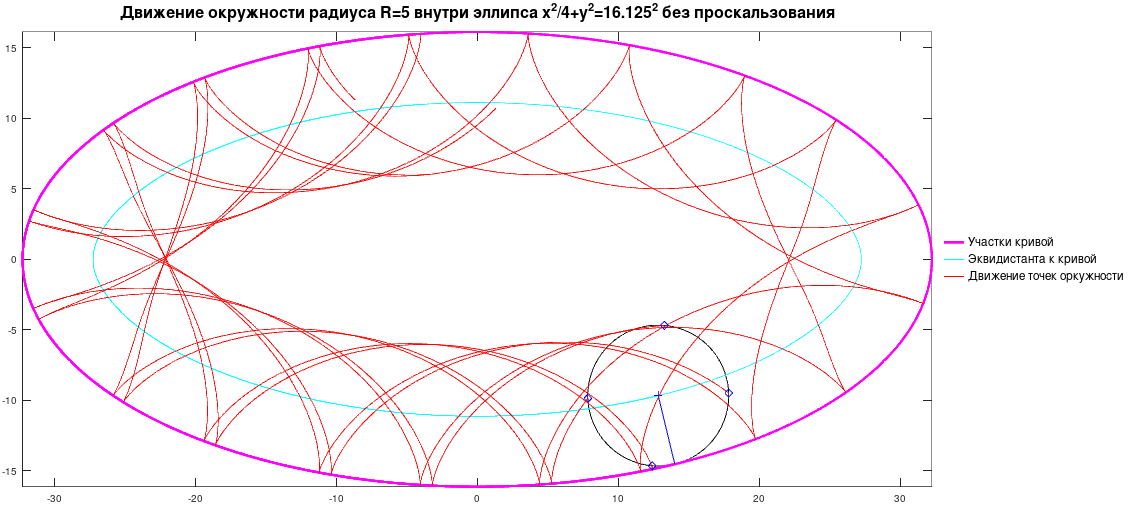
kol3a.mov (986 КиБ) скачан 27 раз(а).
kol3.mov (775 КиБ) скачан 26 раз(а).

An example of visualization of solving a system of 3 equations with 3 variables using the Draghilev method. The system has 6 solutions. All solutions are found for one initial point.

4(x1^2 + x2 - 11)*x1 + 2x1 + 2x2^2 + 2cos(x1) - 14 = 0;
2x1^2 + 2x2 + 4(x2^2 + x1 - 7)*x2 - sin(x2) - 22 = 0;
x1^2 + x3^2 - 1 = 0;


[albumimg]1705[/albumimg]

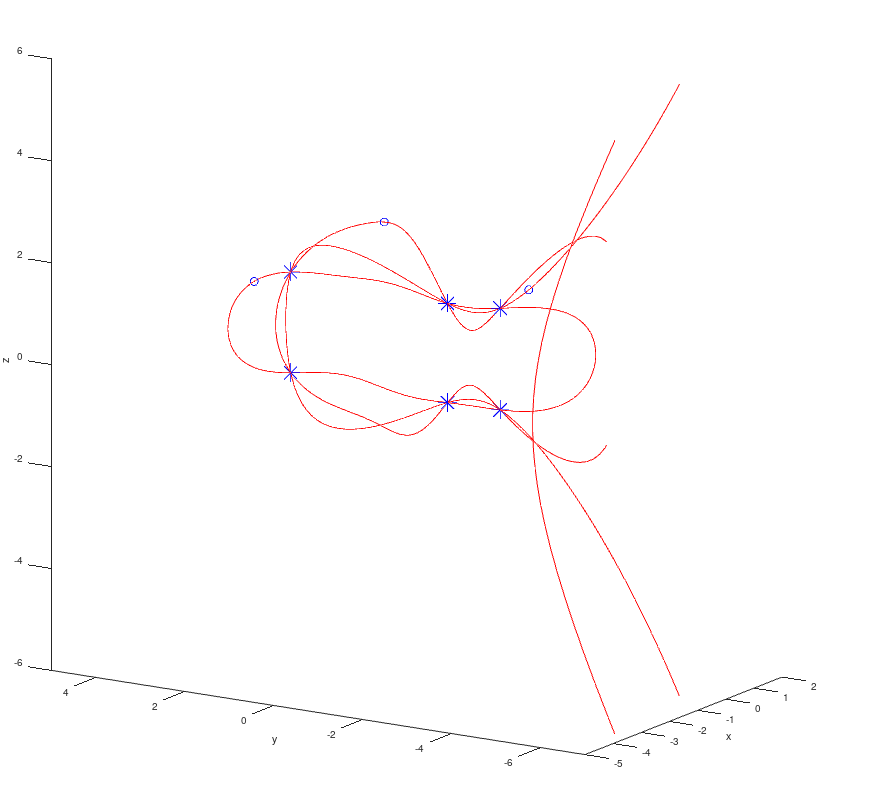
Wrote

An example of visualization of solving a system of 3 equations with 3 variables using the Draghilev method. The system has 6 solutions. All solutions are found for one initial point.

4(x1^2 + x2 - 11)*x1 + 2x1 + 2x2^2 + 2cos(x1) - 14 = 0;
2x1^2 + 2x2 + 4(x2^2 + x1 - 7)*x2 - sin(x2) - 22 = 0;
x1^2 + x3^2 - 1 = 0;


[albumimg]1705[/albumimg]

Solutions to check out:
0.149315 2.877635 0.988708
0.149318 2.877632 -0.988825
-0.231009 -0.888544 -0.972951
-0.083331 -1.981040 -0.996530
-0.083331 -1.981024 0.996514
-0.231007 -0.888540 0.972950

Some initial points:
-3.6100e-01 3.3820e+00 8.4200e-01
-2.0000e-02 -2.5860e+00 1.4310e+00
9.5000e-01 1.2780e+00 2.0150e+00

In the figure, the solutions are shown with an asterisk, the red curves are obtained when different initial conditions are given.